
Design Examples using ProCAP
ProCAP Low-Pass Cross Coupled Filter
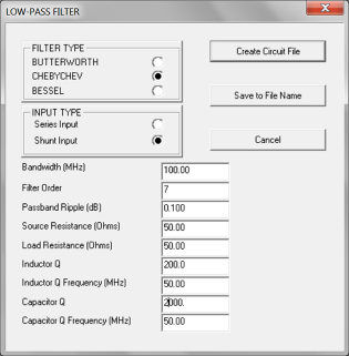
Before selecting the filter design, it is necessary to select the tab labeled Units so that the design uses the desired units for the filter design. The design starts with selecting the tab labeled ‘Design’ and the selection of LC Filt. This brings up a menu for selecting the type of filter: Low Pass, Band-Pass, High-Pass or Band-Stop. In this case the lowpass is selected and a menu appears for input of the design parameters. Upon selecting the type of design a menu appears for placing the desired design parameters. Selecting the tab “Create Circuit File” results in the nodal design appearing in the ProCAP window.
Initially every component has a question mark which were removed except for the first and last capacitor. Then a cross coupled capacitor was added from the first to the last node with a value of 2 pF. Without the capacitor, the solid red line is shown. With the capacitor, the dotted line is shown.
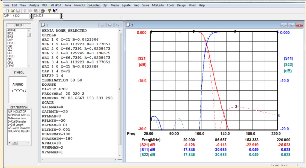
It may be seen that cross-coupling causes some loss reduction out-of-band. Usually placing the cross coupled element to an internal node will reduce the increase in the out-of-band loss. The capacitor labeled C1 was modified to improve return loss. Cross coupling may be made between any two nodes and may be done for any filter type.
ProCAP Diplexer
For the Diplexer design, two interdigital filters were designed using Parfil (not all filter types can be imported into ProCAP): one tuned GPS L1 (1575.42 MHz) and one tuned for L2 (1227.6 MHz). Parfil provides for selection in Parfil of the ProCAP file for import into ProCAP. These filters were combined as shown in Figure 1. The lines from the input to the filters is approximately l/4. The length may be computed from the Smith chart for the L1 filter. The S11 plot is shown in Figure 2. Notice that at the L2 frequency (1223MHz) the angle is at 148 degrees .
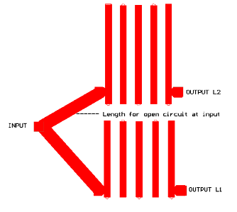
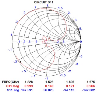
Figure 1. Diplexer layout for filters at L2 and L2 Figure 2. Input S11 for L1 filter
Notice that at the L1 frequency the reflection angle is 148 degrees at the L2 frequency. This means in order to rotate clockwise to an open circuit the line from L1 would need to be (180 + 32)/2 degrees long. For the L1 filter (not shown), the length require for the Line from L1 to the open circuit is 172 degrees and thus the length would be 172 /2 degrees. To create the actual design the lengths and widths of these lines would be optimized for minimum return loss. The measured performance of the diplexer is shown in Figure 3.
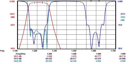
Figure 3. Loss and return loss for Diplexer with the L2 filter selected.
Notice that the return Loss for both filters is shown.
Using this design approach a multiplexer may be designed with as many as 30 filters. Shown in Figure 4 is the performance of a 12 filter multiplexer with the 40 MHz filter selected. In this case the filters not selected are terminated with 50 ohms.
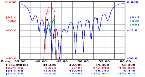
Figure 4. Multiplexer for 12 filters with the 40 MHz filter selected.
The following shows the ProCAP partial data input for analyzing the diplexer.
MEDIA STRIPL ER=2.2 B=0.2 Th=0.0014 Loss_Tan=0.001 Loss_Fact=1 Rough=50
CKTBLK
STE 2 3 1 W1=0.09969 W2=0.09969 W3=0.09969
SCN5 3 4 5 6 7 8 9 10 11 12 W=0.09969 S1=S12 S2=0.1388 S3=0.1388 S4=S12 L=0.193
SCN5 13 2 14 5 15 7 16 9 17 18 W=0.09969 S1=S12 S2=0.1388 S3=0.1388 S4=S12 L=1.372
SLI 13 19 W=0.09969 L=?0.0148316
SLI 17 20 W=0.09969 L=?0.0168162
STE 18 11 51 W1=0.09969 W2=0.09969 W3=0.09969
SVH 4 0 RAD=0.0325
SEN 6 0 W=0.09969
SVH 8 0 RAD=0.0325
SEN 10 0 W=0.09969
SVH 12 0 RAD=0.0325
SEN 19 0 W=0.09969
SVH 14 0 RAD=0.0325
SEN 15 0 W=0.09969
SVH 16 0 RAD=0.0325
SEN 20 0 W=0.09969
STE 22 23 21 W1=0.09993 W2=0.09993 W3=0.09993
SCN5 23 24 25 26 27 28 29 30 31 32 W=0.09993 S1=S1 S2=0.1551 S3=0.1551 S4=S1 L=0.1201
SCN5 33 22 34 25 35 27 36 29 37 38 W=0.09993 S1=S1 S2=0.1551 S3=0.1551 S4=S1 L=1.088
SLI 33 39 W=0.09993 L=?0.00938354
SLI 37 40 W=0.09993 L=?0.0082533
STE 38 31 52 W1=0.09993 W2=0.09993 W3=0.09993
SVH 24 0 RAD=0.0325
SEN 26 0 W=0.09993
SVH 28 0 RAD=0.0325
SEN 30 0 W=0.09993
SVH 32 0 RAD=0.0325
SEN 39 0 W=0.09993
SVH 34 0 RAD=0.0325
SEN 35 0 W=0.09993
SVH 36 0 RAD=0.0325
SEN 40 0 W=0.09993
SLI 53 52 W=?0.186531 L=?1.29683
SLI 53 51 W=?0.197707 L=?1.01501
DEF3P 53 1 21
TERMINATION 50 50 50
EQUATE
S12=?0.12
S1=?0.138
FREQ(GHz) 1.1 1.7 0.003
MARKERS 1.2 1.25 1.55 1.6
ProCAP Lange Couplers
Design of three Lange coupler couplers are described: original Lange coupler, Lange coupler unfolded with 4 lines, and a Lange coupler with 6 lines. These are shown in Figures 1 –3. The performance of the unfolded coupler is nearly identical with that of the original coupler design.
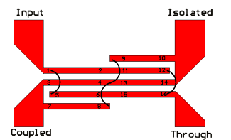
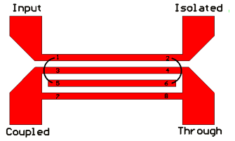
Figure 1. Original Lange coupler
Figure 2. Unfolded Lange coupler 4-line
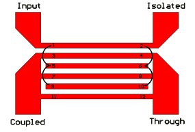
Figure 3. Unfolded Lange coupler 6-line

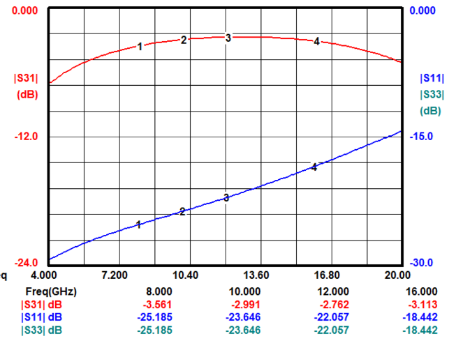
Figure 4. Lange coupler unfolded showing direct path output Figure 5. Lange coupler unfolded showing coupled path output
The following shows the ProCAP partial data input for analyzing the coupler.
MEDIA MSTRIP ER=9.6 H=0.01 CH=0.1 Th=0.0002 Loss_Tan=0.0001 Loss_Fact=1 Rough=55
CKTBLK
MCN4 1 2 3 4 1 2 3 4 W=W S1=S1 S2=S S3=S1 L=L
RES 4 0 R=50
DEF3P 1 2 3
TERMINATION 50 50 50
EQUATE
S=?0.00125
S1=?0.0015
W=0.0026
L=0.098
FREQ(GHz) 4 20 0.12
MARKERS 8 10 12 16
SCALE
ProCAP Ceramic Tapped Combline Filter
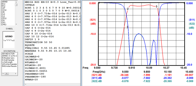
Using Parfil, A tapped rod coupled combline filter as designed a 10 GHz as shown in the data below. In order to not have too small a filter, the resonator length was chosen as 80 degrees. This design uses Aluminum oxide substrate with a loss tangent of .0001. The rods are formed in the ceramic block by drilling and plating the drilled walls of the ceramic block. The line width was selected at a fixed width of 0.06 “.
Tapped Round Rod Combline Filter
10.000 GHz CENTER FREQUENCY 0.30000 GHz BANDWIDTH
0.0500 dB RIPPLE 5 POLES
0.3000 INCHES GROUNDPLANE SPACING 10.000 DIELECTRIC CONSTANT
35.120 OHMS INTERNAL IMPEDANCE
50.000 OHMS INPUT LINE IMPEDANCE 0.0273 INCHES INPUT LINE WIDTH
50.000 OHMS OUTPUT LINE IMPEDANCE 0.0273 INCHES OUTPUT LINE WIDTH
0.0131 INCHES INPUT TAP TO SHORT 0.0131 INCHES OUTPUT TAP TO SHORT
80.000 DEGREES RESONATOR LENGTH 0.0002 nH INDUCTANCE OF END CAP
0.0500 INCHES DISTANCE TO SIDEWALL 0.0100 INCHES DIAMETER OF INPUT LINE
10.000 DIELECTRIC CONSTANT EVEN MODE 10.000 DIELECTRIC CONSTANT ODD MODE
0.0100 INCHES LINE DIA SIDEWALL-TAP
SECT ELEMENT ZOE ZOO LENGTH WIDTH GAP END CAP
NUMB VALUE OHMS OHMS INCHES INCHES INCHES pF
1 0.9984 43.182 0.0828 0.0604 0.0770
34.207 0.1615
2 1.3745 42.899 0.0828 0.0595 0.0794
35.443 0.1798
3 1.8283 42.419 0.0828 0.0587 0.0787
35.443 0.1798
4 1.3745 42.899 0.0828 0.0595 0.0794
34.207 0.1615
5 0.9984 43.182 0.0828 0.0604 0.0770
The design results from Parfil are shown in the plot of Figure 1. Losses were not included
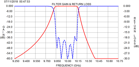
Figure 1. Tapped combline filter loss and return loss vs. frequency
From Parfil, the ProCAP file is imported as shown in Figure 2. The ProCAP plotted output also shows the initial computed performance. The discrepancy is due to the transfer from synthesis to analysis. This usually results in small changes in the capacitances computed. In ProCAP, an optimization was performed in which the capacitances are changed while optimizing for return loss.
After optimizing the capacitances, the resultant frequency response is shown in Figure 3.
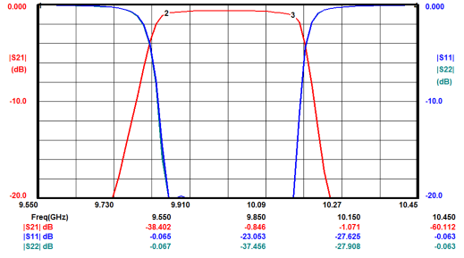
Figure 3. Frequency response after optimizing capacitances.
The changes in capacitances are .0012 pF, .00456pF and .00356pF. These represent changes less than 5 percent. Some of the 1.8% is due to slightly tuning the center frequency. In addition for optimum performance the distance to the tap point was shortened by 10 percent. This frequency response plot includes losses which are less than 1dB except at one band edge. The line spacing and widths were not changed. Generlly better results are obtained from interdigital filters
ProCAP Balanced Amplifier
A Balanced amplifier is one in which two amplifiers are used with hybrid couplers at both the input and output of the two amplifiers. This result in greatly improved input and output impedances. The hybrid couplers could be Lange couplers or the more traditional branch line hybrid couplers. This is illustrated in Figures 1 and 2.
Figures 3 and 4 show the performance of the branch Line hybrid for direct and coupled outputs.
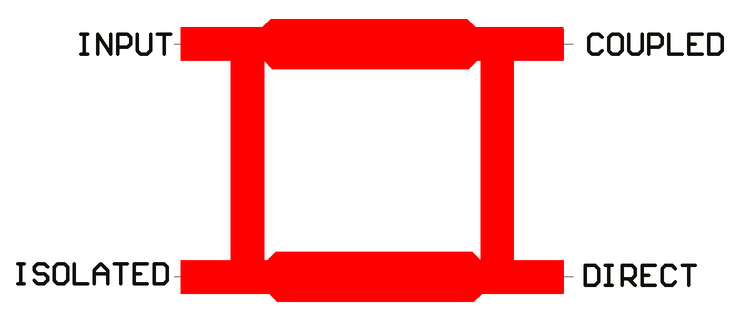
Figure 1. Branch Line Hybrid
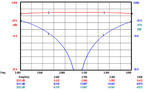
Figure 2. Lange Coupler
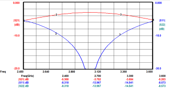
Figure 3. Branch Line hybrid direct output. Figure 4. Branch Line hybrid coupled output
The data used for the calculations is as follows:
MEDIA MSTRIP ER=2.2 H=0.03125 CH=0.25 Th=0.0014 Loss_Tan=0.001 Loss_Fact=1 Rough=50
CKTBLK
MLI 1 2 W=W1 L=L1
MLI 1 3 W=W2 L=L2MLI 2 4 W=W2 L=L2
MLI 3 4 W=W1 L=L1
RES 2 0 R=50
DEF3P 1 3 4
TERMINATION 50 50 50
EQUATE
W1=0.0938
W2=0.1538
W3=0.0938
L1=0.7168
L2=0.7058
FREQ(GHz) 2.4 3.6 0.02
MARKERS 2.4 2.7 3.3 3.6
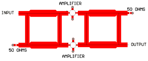
Figure 5: Balanced hybrid coupled amplifier circuit illustration
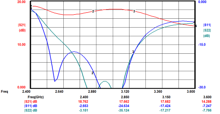
Figure 6. Balanced amplifier circuit performance using branch line hybrids
The output for this circuit is shown in Figure 6. The return loss is considerably improved over a single amplifier. For wide bandwidth circuits, the Lange coupler would be used.